Top-down tree & lightcut cost

Over the last 2 weeks I:

• Implemented a top down light tree builder & experimented with some modifications to the heuristic used
• Estimated the cost for several parts of the lightcuts algorithm in a few scenes

The top-down tree building algorithm I implemented is a simple greedy (based on the heuristic) approach like the ones used for ray intersection acceleration structure building with SAH. To implement this efficiently for a significant number of lights (ex. 100k) poses some problems for the cone angle term in the heuristic used by the authors of the Lightcuts paper. Currently I calculate this angle for all split candidates in a single sweep over which obviously results in suboptimal angles. Another restrictions in the current top-down approach is that all lights are split in 2 non-overlapping (spatially) groups. Most of the time this poses no problems and has the nice side-effect of clustering lights that fill their bounding volume a lot better then cluster formed in the bottom up approach.
After visualizing some of the trees resulting from the top-down and bottom-up approaches with the heuristic as proposed in the lightcuts paper it was clear that the clusters formed for indirect lights are sub-optimal. These clusters tend to extend into empty space instead of following the geometry more closely. To suppress this phenomenon I added the size of the bounding in the direction of the normal as a term to the heuristic. I also changed the coefficient for the angle and new term from the squared diagonal length of the entire scene to the squared diagonal length of the current box being split. Using this heuristic in the conference scene with a glossy floor resulted in a modest improvement for the cut size (15%) for a similar tree build time.

After being suggested in the meeting last week, I also tried to estimate the cost for several parts of the lightcuts algorithm. The total render time can be split as:

Ttot = Teval + Tbound + Titer

whith

• Ttot: the total render time


• Teval: the time required for evaluating the clusters (i.e. shadow ray, bsdf & geometric term)


• Tbound: the time for evaluating the upper bounds for the clusters


• Titer: the other time (o.a. pushing/popping on the priority queue)

To estimate these I rendered the same scene several times:

• lightcuts (Ttot)


• lightcuts + an extra evaluation of the resulting cut (Ttot + Teval)


• lightcuts + an extra evaluation of all bounds which also requires storing these in a list during cut calculation (Ttot + Tbound)


• lightcuts + resulting cut + bounds (Ttot + Teval + Tbound)

The scenes used where the conference scene and the statues scene (once diffuse only and once diffuse & glossy). For all the scenes Titer is around 20% of the total time, the cost for the bounds varies a bit more however: 35% for the conference scene (cos light sources have a more expensive bound), 12% for the diffuse statues scene (directional light bound is trivial) and 21% for the glossy statues scene (the glossy bound is more expensive then a diffuse bound). The resulting Teval's are respectively 43%, 66% and 58% (same order as before) so a modest improvement is possible if (a part of) the cuts could be reused. Reusing cuts could be done in a similar way as the reconstruction cuts algorithm proposed in the paper but by completely evaluating (and if necessary refining) the cut, the result will be identical to the lightcuts result. The reconstruction cuts approach however could blur or miss some fine details (ex. shadow boundaries).

Upper bounds & visualization tool

Here is a short overview of what I did over the past weeks:

• fix bugs in visibility bounds
• create a visualization tool (light tree, light cuts & precalculated visibility)
• calculate optimal visibility bounds (i.e. perfect visibility estimation in bounds)

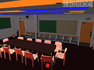
I finally found some major bugs in my visibility precalculation step (o.a. a wrong interval for the parameter of the rays). To test the new implementation I rendered the conference scene. This scene is lit by a number of large area light sources on the ceiling resulting in very soft shadows (i.e. no trivial occlusion).
The general settings used where:

• samples/pixel: 1
• resolution: 640x480
• #light sources: 3000 (allows calculating a reference solution in an acceptable time frame)
• maximum cut size: 1000

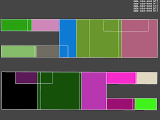
Rendering this scene with the lightcuts algorithm results in an average lightcut size of 126 and requires 3:50s. A relatively large fraction of this time (>50%) is consumed by the highly occluded pixels under the chairs and table. Rendering this scene using an optimal upper bound on the visibility (i.e. perfect detection of occluded clusters) results in an average cut size of 70 (44% less) so a significant improvement is possible. Rendering the scene using an estimated upper bound on visibility results in an average cut size of 95 (25% less then lightcuts) and a render time of 3:04s. Here the upper bound was estimated by dividing the scene in a grid of 100000 cells, selecting for each cell a number of clusters based on their solid angle (55 on average) and finally sampling each of these clusters with up to 1000 rays to assure it is occluded. This preprocess step is more expensive (about 5:00s) then actually rendering the image (with the given settings) but can be reused for arbitrary view points and/or image resolutions. The first image shows the relative reduction in cut size of this solution w.r.t. the lightcuts solution:Because only an upper bound is used, there is no improvement (i.e. 0% less cut size) but most of the occluded regions have a reduction of about 50% or more. The grid that was used for the visibility calculation is also clearly visible. The next image shows the relative distance from the optimal solution (i.e. (optimal cut - estimate cut)/optimal cut):Here it is clearly visible that some occlusion cannot be easily detected by using a grid subdivision: the upper part of the back of the chairs is occluded by the chair itself. The occluding geometry in this case is located at a very low angle w.r.t. the occluded points. But the cells used to calculate occlusion extend to a significant distance away from the chair and is only partly occluded. This could be solved by using smaller cells or taking geometric orientation of the surfaces into account for calculating visibility (ex. start the rays from a plane aligned to the local geometry instead of from within a fixed bounding box).

Over the past few weeks I also implemented (after suggestion by my counselor) a tool that allows interactive inspection of: the light tree, the light cuts used for each points and the visibility bounds precalculated for each cell. These are all visualized by drawing the scene and some bounding boxes (representing the data) with opengl. For the light tree all bounding boxes at a specific level of the hierarchy are shown. The following scene shows the 5th (out of 15) level of the light hierarchy calculated for the conference scene:
It is a top view of the 4 rows of light sources on the ceiling where each cluster is colored in a different color and an indication of the edges of these clusters. It is immediately apparent that an improvement is possible: there is a significant overlap between the clusters and the cluster sizes are quiet dissimilar even though all point light sources have the same intensity and orientation and are evenly distributed over the light sources. The cause is most likely the greedy bottom up approach used to cluster light sources which will produce the best cluster low in the hierarchy and possibly worse (due to its greedy nature) near the top. Intuitively this is not optimal as the lower part of the tree is unimportant for most light cuts and the upper part is used by all light clusters.
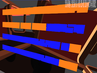
The next picture shows the visualization of the precalculated visibility for the selected cell under the chair (indicated by a red box):
The blue colored light clusters are detected as occluded and the orange onces as potentially unoccluded. The quality of this specific bound is better visible when these clusters are rendered from the perspective of the cell (disabling the depth test on the visibility data) as seen in the following image:
Finally the light cut calculated, on the same position as the previous image, using the lightcuts algorithm and the extension with an upper bound on visibility is shown in the following 2 images (each cluster has an individual color):


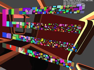
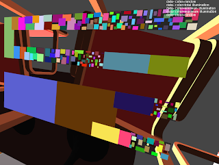
A clear reduction in the number of light clusters used is visible (from about 550 to 200).

Correction

At the end of my previous post I stated that the upper bound was responsible for most of the improvement w.r.t. render time. After re-running the test, it seems this statement was based on a typo. The render times when only an lower or upper bound on visibility are used are 4:56s and 4:50s so the improvement is about the same.

First visibility bounds

It has been some time since my last post. This is mostly due to preparations for my presentation about 1.5 weeks ago. In the time frame between 1.5 weeks ago and now I also had some other work (other presentation, ...) which further reduced the time left to work on my thesis.
Now that is out of the way, here is what I did do:

• read some more papers on conservative visibility bounds
• implement basic visibility bounds

The papers I read where:

• Voxel Occlusion Testing: A Shadow Determination Accelerator for Ray Tracing - Woo A. & Amanatides J. (1990)
• A Survey of Visiblity for Walkthrough Applications - Cohen-Or D., Chrysanthou Y., Claudio T. S. (2000)

These papers mostly confirmed my previous remark that most of the proposed algorithms can only be used in a preprocessing step (storing the result in some kind of spatial structure) to amortize their cost over a large number of pixels and/or frames.

After reading these papers I implemented a basic lower and upper bound on the visibility. To detect clusters that are completely unoccluded (i.e. the points where a lower bound can be calculated) I used the shaft culling algorithm mention in my previous post. To verify whether a specific shaft is empty, I use a bounding volume hierarchy that is constructed during the preprocessing phase to quickly reject most primitives. The test is however conservative because it will only succeed if the entire bounding box is outside the shaft and no real primitives are tested against the shaft. Because testing a shaft is still quiet expensive, it is only used for lightcluster in the upper part of the hierarchy. In the results presented at the end of this post such test is only performed up to level 4 of the light tree which limits the number of shafts per lightcut to 31.
For detecting cluster that are completely occluded I currently use a very simple approach where one occlusion value (all lights are either occluded or not) is calculated for all cells in a regular grid. To estimate the occlusion value, a number of random rays are shot between both bounding boxes and tested for occlusion. In the results presented at the end, the scene is subdivided in 1 million cells which each use up to 1000 rays for the estimate. It is however important to notice that most cells only use a small fraction of these rays because once an unoccluded ray is found, the cell is categorized as not unoccluded. In the scene used less then 1% of maximum number of rays (1 billion) is actually tested.

To test this implementation I used one of the scenes used by Peter Shirley for testing radiosity. The scene consists of a room with a table with chairs lit by single area light source on the ceiling. The first and second pictures show the result of rendering this scene using regular lightcuts and lightcuts extended with the implementation described above and the following settings:

• resolution: 640x480
• samples/pixel: 4
• area light approx.: 1024 point lights
  
• render-machine: AMD X2 3800+ (single core used) with 1GB ram
• lightcuts rel. error: 2%
• max. cut size: 1000
  

The time required for these virtually indistinguishable images was 4:13s and 9:03s (50% reduction) with an average cut size of 46 and 126 (60% reduction). The reduction in render time is smaller due to the calculations involved (shaft culling & calculating lower bounds).


The following 2 images show the relative error (using a reference solution) for each pixel. The average relative error is 0.26% and 1.19% respectively. As expected using more tight bounds results in a relative error closer to the 2% target error.


The final image shows the relative reduction in cut size for each pixel. This reduction is largest in the occluded regions where the lightcuts algorithm uses the maximum cut allowed (i.e. 1000) and the extended implementation uses a minimal cut (i.e. 1). To verify that the upper bound on its own is not the major contributor to the improvement (i.e. making the lower bound useless in this scene) I rendered this scene using only a lower and only an upper bound on the visibility. The resulting cut sizes are 82 if only a lower bound on the visibility is used and 91 if only an upper bound on the visibility is used. The upper bound is however responsible for most of the reduction in render time.

Next step?

Besides completing my Lightcuts implementation during the last week, I have searched for possible next steps in my thesis.
One possible extention to the Lighcuts algorithm, as already identified in the paper, is the addition of bounds on the visibility term. I have read a number of papers on this subject:

• Shaft Culling For Efficient Ray-Cast Radiosity - Haines E. & Wallace J. (1991)
  
• ShieldTester: Cell-to-Cell Visibility Test for Surface Occluders - Navazo I., Rossignac J., Jou J. & Shariff R. (2003)
• Conservative Volumetric Visibility with Occluder Fusion - Schaufler G., Julie D., Decoret X. & Sillion F. (2000)

and found one other paper that might be interesting:

• Ray Space Factorization for From-Region Visibility - Leyvand T., Sorkine O. & Cohen-Or D. (2003)

All these techniques have fairly large disadvantages in the context of the calculation of bounds on the visibility. For example the first paper can only guarantee total occlusion if it is cause by a single object (i.e. 1 triangle). In practice this will only work well if there are a number of large polygons in the scene. There do exist a number of extensions that can detect the aggregate occlusion of a number of objects by for example reconstruction larger planes from a number of smaller triangles. The second paper is only applicable to triangles and needs structural information about the meshes (ex. neighbors of a triangle). In the last paper, the scene is discretized which inevitably leads to missing small features (ex. small holes).
Further more all these techniques are quite expensive. This means they can only be used in very selective cases during lightcut calculation or only during a pre-processing phase.

The shaft-culling technique is able to efficiently detect clusters that are totally visible. This could be used to calculate lower bounds on the cluster contribution which results in better error estimates and lower cut sizes.

A totally different approach is to drop the deterministic nature of the lightcuts algorithm and use inexact estimates of the visibility. One possibility would be to first calculate a cut using the bounds and then construct a pdf over the resulting clusters using their estimated contribution. The total contribution of all lights can the be estimated by generating a number of samples from this pdf.
Ideally the user should be able to control the amount of determinism (i.e. the solution goes from the lightcuts solution to totally stochastic according to a parameter).

Lightcuts implementation

During the past week I completed my lightcuts implementation. Concretely this means I added cosine weighted point lights and directional lights (clustering & bounds), a bound for the Blinn microfacet distribution and support for global illumination using the Instant Global Illumination algorithm as implemented in the igi plugin for pbrt.
All of the following pictures where rendered using this updated implementation on my Core2 Duo T7100 system using 4 samples per pixel. The first picture is once again the cornell box but now using 1024 cosine weighted lights instead of omni directional lights with a maximum relative error of 2%. The total render time for this picture was 227s and the average cut size was 104.



The second picture shows a modified cornell box with glossy objects and global illumination. The total number of light sources used was 760000 which were mostly for the indirect light. The required time was 632s and the average cut size 206.



The final picture shows a glossy dragon statue lit by the grace environment map. This environment map was approximated by 256000 directional lights distributed evenly over the entire sphere of directions. The total render time was 1557s and the average cut size 218.

Total illumination misinterpretation

After some more testing and re-reading the lightcuts paper I have come to the conclusion that the calculation of the total radiance estimate (used to determine what errors are allowed) in my implementation differs from the one used by the authors of the lightcuts paper. As described in my previous post, I used the maximum total illumination as an estimate of the total illumination. While the authors of the lightcuts papers do not state so explicitly they most likely used the current lightcut approximation as an estimate for the total illumination. This estimate is by definition always less then the maximum total illumination and will thus result in a lower allowed error per cluster.
Using the current lightcut approximation generally improves the estimate but is especially important in highly occluded regions because the difference with the maximum total illumination is largest here. I re-rendered the cornell box scene using this new total illumination estimate:

• resolution: 512x512
• samples/pixel: 4
• pixel filter: gaussian
• area light approx.: 1024 omnidirectional lights
• render-machine: Core2 Duo T7100 (single core used) with 2GB ram

As you can see I used a different machine so the timings are not comparable to my previous test. The first picture shows the reference solution (795s). The following 2 pictures show the lightcuts approximation with a respective maximum relative error of 2% (182s) and 5% (107s). Both of the lightcuts pictures used a maximum cut size of 1024 (i.e. all lights) which is always used in the completely occluded regions due to the new total illumination estimate being 0. The average cut sizes where 119 and 73.




Like in my previous test, the final 2 pictures show the relative error. It is clear that the total illumination estimate used by the authors of the lightcuts paper is a lot better then using the maximum total illumination: the relative error is even in the highly occluded places very close to the target (avg: 0.36% and 0.95%; max: 2.1% and 3.5%).

Lightcut error clarification

The error images in my previous post are the relative error of the lightcuts image w.r.t. the reference image (i.e. abs(lightcuts - reference) / reference). This error differs from the error bound used in the lightcuts algorithm because the reference solution is obviously not available during the lightcut calculations. The lightcuts algorithm uses an upper bound on the total illumination (further referred to as maximum total illumination or mti) to determine whether the maximum error for a particular cluster is acceptable (i.e. it is smaller then some percentage of the mti). So the lightcuts algorithm gives no real guarantee w.r.t. the real relative error. Such a guarantee would require using a minimum total illumination which is a lot harder then a maximum because a decent lower bound on the visibility term is necessary.
During cut refinement the estimate of the mti is also improved using the bounds computed for the refined clusters. This means that not only the error bounds on the individual clusters drops, but also the mti and thus the maximum allowed error.
In pseudo-code the lightcut algorithm is something like this:

rootUpperBound = calc. upper bound root cluster
mti = rootUpperBound
root.maxerr = rootUpperBound
cut = [root]
while(largest cluster error in cut > some% of mti) {
  cluster = remove cluster from cut with largest error
  left = cluster.leftchild
  right = cluster.rightchild
  leftUpperBound = calc. upper bound left cluster
  rightUpperBound = calc. upper bound right cluster
  if(left is leaf)
    left.maxerr = 0;
  else
    left.maxerr = leftUpperBound
  if(right is leaf)
    right.maxerr = 0
  else
    right.maxerr = rightUpperBound
  mti -= cluster.maxerr
  mti += leftUpperBound + rightUpperBound
  cut = [cut left right]
}

The lowering of the mti can result in some unexpected effects like a reduction in cut size for occluded pixels if the number of lights increases. This is caused by a cascade effect if too few light sources are used at these occluded pixels. At some point during cut refinement a leaf node is reached. Because the point is occluded, the mti will be significantly reduced (the previous node still had a non-zero upper bound). This results in more nodes that need to be refined which again results in new leaf nodes.
The use of the mti instead of the reference image in the calculation of the maximum acceptable error also explains the large relative errors in shadow boundaries as visible in the error images of my previous post. In the highly occluded regions the mti is significantly higher then the real illumination due to the poor visibility bound (i.e. everything is visible), so the lightcuts algorithm will allow too large errors.

First render

Last weekend I implemented a light tree construction algorithm for omnidirectional lights, bounds for omnidirectional lights and a trivial bound for the cos term (i.e. 1) and the diffuse brdf (this brdf is already a constant). Using this basic implementation I rendered some pictures of the famous cornell box. The setup for all pictures was as follows:

• resolution: 512x512
• samples/pixel: 4
• pixel filter: gaussian
• area light approx.: 256 omnidirectional lights arranged in a regular grid
• render-machine: AMD X2 3800+ (single core used) with 1GB ram

The first picture shows a reference solution (i.e. sampling all lights) and rendered for for 234s. The next 2 pictures were rendered using the basic implementation with a maximum relative error of respectively 1% and 2%. These images rendered for 204s and 101s with a average cutsizes of 157 and 72 respectively.



The final 2 pictures show the relative error between the reference picture and the pictures rendered using the lightcuts algorithm. There are a few strangely colored pixel due to a division by zero in some (but not all) of the channels. Although the relative error on most pixels is far below the maximum relative error, some pixels (especially in dark regions) have considerably higher relative errors (up to 100% for the 1% relative error image and up to 300% for the 2% relative error image). It is not clear yet whether these are caused by a flaw in the implementation, some numerical issue or something else.

Installation PBRT & inital implementation

Since my last post I have, with no significant problems, installed the latest version of PBRT (1.03) on both Windows & Linux. The installation on the Ludit HPC (cluster) required some more attempts but I eventually got it to work by recompiling the OpenEXR library.
After my first meeting with my couselor earlier this week, I started today with the implementation of the Lightcuts algorithm. Even though I currently do not have a working implementation, I have already progressed quite a bit. The major components that are still missing are: building the light tree & calculation of most of the material/light bounds.

Introduction & study of literature

On this blog you will be able to follow the progress of my master thesis "Advanced Global Illumination using Lightcuts" throughout the year. The goal of this thesis is to implement the Lightcuts algorithm as a plugin for PBRT and compare and evaluate the algorithm.
During the summer holidays I have read the following papers for my study of literature:

• Direct Lighting Calculation by Monte Carlo Integration - Shirley P. & Wang C. (1991)
  
• Monte Carlo Techniques for Direct lighting Calculations - Shirley P., Wang C. & Zimmerman K. (1996)
  
• Adaptive Shadow Testing for Ray Tracing - Ward G. (1994)
• A Light Hiërarchy for Fast Rendering of Scenes with Many Lights - Paquette E., Poulin P. & Drettakis G. (1998)
  
• Instant Radiosity - Keller A. (1997)
  
• Interactive Global Illumination using Fast Ray Tracing - Wald I., Kollig T., Keller A. & Slusallek P. (2002)
  
• A Scalable Approach to Interactive Global Illumination - Benethin C., Wald I. & Slusallek P. (2003)
  
• Instant Global Illumination - Pharr M. (2004)
  
• Interactive Global Illumination in Complex and Highly Occluded Environments - Wald I., Benethin C. & Slusallek P. (2003)
  
• Matrix Row-Column Sampling for the Many-Light Problem - Hasan M., Pellacini F. & Bala K. (2007)
  
• Lightcuts: A Scalable Approach to Illumination - Walter B., Fernandez S., Arbree A., Bala K., Donikian M. & Greenberg D. (2005)
  
• Implementing Lightcuts - Walter B., Fernandez S., Arbree A., Bala K., Donikian M. & Greenberg D. (2005)
• Notes on the Ward BRDF - Walter B. (2005)
• Implementing Lightcuts - Miksik M. (2007)
  
• Multidimensional Lightcuts - Walter B., Arbree A., Bala K. & Greenberg D. (2006)