Sunday, October 12, 2008
Final post
I continued working on my thesis during the second semester but "forgot" to post progress here. Anyway, I am now graduated and you can find my final thesis and 2 papers on my thesis mini-site
Tuesday, December 11, 2007
Top-down tree & lightcut cost
Over the last 2 weeks I:
After visualizing some of the trees resulting from the top-down and bottom-up approaches with the heuristic as proposed in the lightcuts paper it was clear that the clusters formed for indirect lights are sub-optimal. These clusters tend to extend into empty space instead of following the geometry more closely. To suppress this phenomenon I added the size of the bounding in the direction of the normal as a term to the heuristic. I also changed the coefficient for the angle and new term from the squared diagonal length of the entire scene to the squared diagonal length of the current box being split. Using this heuristic in the conference scene with a glossy floor resulted in a modest improvement for the cut size (15%) for a similar tree build time.
After being suggested in the meeting last week, I also tried to estimate the cost for several parts of the lightcuts algorithm. The total render time can be split as:
whith
- Implemented a top down light tree builder & experimented with some modifications to the heuristic used
- Estimated the cost for several parts of the lightcuts algorithm in a few scenes
After visualizing some of the trees resulting from the top-down and bottom-up approaches with the heuristic as proposed in the lightcuts paper it was clear that the clusters formed for indirect lights are sub-optimal. These clusters tend to extend into empty space instead of following the geometry more closely. To suppress this phenomenon I added the size of the bounding in the direction of the normal as a term to the heuristic. I also changed the coefficient for the angle and new term from the squared diagonal length of the entire scene to the squared diagonal length of the current box being split. Using this heuristic in the conference scene with a glossy floor resulted in a modest improvement for the cut size (15%) for a similar tree build time.
After being suggested in the meeting last week, I also tried to estimate the cost for several parts of the lightcuts algorithm. The total render time can be split as:
Ttot = Teval + Tbound + Titer
whith
- Ttot: the total render time
- Teval: the time required for evaluating the clusters (i.e. shadow ray, bsdf & geometric term)
- Tbound: the time for evaluating the upper bounds for the clusters
- Titer: the other time (o.a. pushing/popping on the priority queue)
- lightcuts (Ttot)
- lightcuts + an extra evaluation of the resulting cut (Ttot + Teval)
- lightcuts + an extra evaluation of all bounds which also requires storing these in a list during cut calculation (Ttot + Tbound)
- lightcuts + resulting cut + bounds (Ttot + Teval + Tbound)
Tuesday, November 27, 2007
Upper bounds & visualization tool
Here is a short overview of what I did over the past weeks:
The general settings used where: Because only an upper bound is used, there is no improvement (i.e. 0% less cut size) but most of the occluded regions have a reduction of about 50% or more. The grid that was used for the visibility calculation is also clearly visible. The next image shows the relative distance from the optimal solution (i.e. (optimal cut - estimate cut)/optimal cut):
 Here it is clearly visible that some occlusion cannot be easily detected by using a grid subdivision: the upper part of the back of the chairs is occluded by the chair itself. The occluding geometry in this case is located at a very low angle w.r.t. the occluded points. But the cells used to calculate occlusion extend to a significant distance away from the chair and is only partly occluded. This could be solved by using smaller cells or taking geometric orientation of the surfaces into account for calculating visibility (ex. start the rays from a plane aligned to the local geometry instead of from within a fixed bounding box).
Over the past few weeks I also implemented (after suggestion by my counselor) a tool that allows interactive inspection of: the light tree, the light cuts used for each points and the visibility bounds precalculated for each cell. These are all visualized by drawing the scene and some bounding boxes (representing the data) with opengl. For the light tree all bounding boxes at a specific level of the hierarchy are shown. The following scene shows the 5th (out of 15) level of the light hierarchy calculated for the conference scene: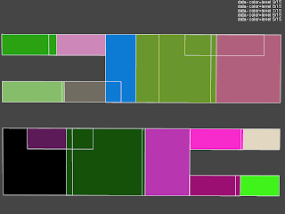
It is a top view of the 4 rows of light sources on the ceiling where each cluster is colored in a different color and an indication of the edges of these clusters. It is immediately apparent that an improvement is possible: there is a significant overlap between the clusters and the cluster sizes are quiet dissimilar even though all point light sources have the same intensity and orientation and are evenly distributed over the light sources. The cause is most likely the greedy bottom up approach used to cluster light sources which will produce the best cluster low in the hierarchy and possibly worse (due to its greedy nature) near the top. Intuitively this is not optimal as the lower part of the tree is unimportant for most light cuts and the upper part is used by all light clusters.
The next picture shows the visualization of the precalculated visibility for the selected cell under the chair (indicated by a red box):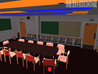
The blue colored light clusters are detected as occluded and the orange onces as potentially unoccluded. The quality of this specific bound is better visible when these clusters are rendered from the perspective of the cell (disabling the depth test on the visibility data) as seen in the following image: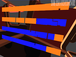
Finally the light cut calculated, on the same position as the previous image, using the lightcuts algorithm and the extension with an upper bound on visibility is shown in the following 2 images (each cluster has an individual color):
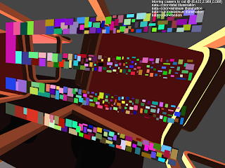
A clear reduction in the number of light clusters used is visible (from about 550 to 200).
- fix bugs in visibility bounds
- create a visualization tool (light tree, light cuts & precalculated visibility)
- calculate optimal visibility bounds (i.e. perfect visibility estimation in bounds)
The general settings used where:
- samples/pixel: 1
- resolution: 640x480
- #light sources: 3000 (allows calculating a reference solution in an acceptable time frame)
- maximum cut size: 1000
 Because only an upper bound is used, there is no improvement (i.e. 0% less cut size) but most of the occluded regions have a reduction of about 50% or more. The grid that was used for the visibility calculation is also clearly visible. The next image shows the relative distance from the optimal solution (i.e. (optimal cut - estimate cut)/optimal cut):
 Here it is clearly visible that some occlusion cannot be easily detected by using a grid subdivision: the upper part of the back of the chairs is occluded by the chair itself. The occluding geometry in this case is located at a very low angle w.r.t. the occluded points. But the cells used to calculate occlusion extend to a significant distance away from the chair and is only partly occluded. This could be solved by using smaller cells or taking geometric orientation of the surfaces into account for calculating visibility (ex. start the rays from a plane aligned to the local geometry instead of from within a fixed bounding box).
Over the past few weeks I also implemented (after suggestion by my counselor) a tool that allows interactive inspection of: the light tree, the light cuts used for each points and the visibility bounds precalculated for each cell. These are all visualized by drawing the scene and some bounding boxes (representing the data) with opengl. For the light tree all bounding boxes at a specific level of the hierarchy are shown. The following scene shows the 5th (out of 15) level of the light hierarchy calculated for the conference scene:

It is a top view of the 4 rows of light sources on the ceiling where each cluster is colored in a different color and an indication of the edges of these clusters. It is immediately apparent that an improvement is possible: there is a significant overlap between the clusters and the cluster sizes are quiet dissimilar even though all point light sources have the same intensity and orientation and are evenly distributed over the light sources. The cause is most likely the greedy bottom up approach used to cluster light sources which will produce the best cluster low in the hierarchy and possibly worse (due to its greedy nature) near the top. Intuitively this is not optimal as the lower part of the tree is unimportant for most light cuts and the upper part is used by all light clusters.
The next picture shows the visualization of the precalculated visibility for the selected cell under the chair (indicated by a red box):

The blue colored light clusters are detected as occluded and the orange onces as potentially unoccluded. The quality of this specific bound is better visible when these clusters are rendered from the perspective of the cell (disabling the depth test on the visibility data) as seen in the following image:

Finally the light cut calculated, on the same position as the previous image, using the lightcuts algorithm and the extension with an upper bound on visibility is shown in the following 2 images (each cluster has an individual color):


A clear reduction in the number of light clusters used is visible (from about 550 to 200).
Tuesday, November 6, 2007
Correction
At the end of my previous post I stated that the upper bound was responsible for most of the improvement w.r.t. render time. After re-running the test, it seems this statement was based on a typo. The render times when only an lower or upper bound on visibility are used are 4:56s and 4:50s so the improvement is about the same.
Monday, November 5, 2007
First visibility bounds
It has been some time since my last post. This is mostly due to preparations for my presentation about 1.5 weeks ago. In the time frame between 1.5 weeks ago and now I also had some other work (other presentation, ...) which further reduced the time left to work on my thesis.
Now that is out of the way, here is what I did do:
After reading these papers I implemented a basic lower and upper bound on the visibility. To detect clusters that are completely unoccluded (i.e. the points where a lower bound can be calculated) I used the shaft culling algorithm mention in my previous post. To verify whether a specific shaft is empty, I use a bounding volume hierarchy that is constructed during the preprocessing phase to quickly reject most primitives. The test is however conservative because it will only succeed if the entire bounding box is outside the shaft and no real primitives are tested against the shaft. Because testing a shaft is still quiet expensive, it is only used for lightcluster in the upper part of the hierarchy. In the results presented at the end of this post such test is only performed up to level 4 of the light tree which limits the number of shafts per lightcut to 31.
For detecting cluster that are completely occluded I currently use a very simple approach where one occlusion value (all lights are either occluded or not) is calculated for all cells in a regular grid. To estimate the occlusion value, a number of random rays are shot between both bounding boxes and tested for occlusion. In the results presented at the end, the scene is subdivided in 1 million cells which each use up to 1000 rays for the estimate. It is however important to notice that most cells only use a small fraction of these rays because once an unoccluded ray is found, the cell is categorized as not unoccluded. In the scene used less then 1% of maximum number of rays (1 billion) is actually tested.
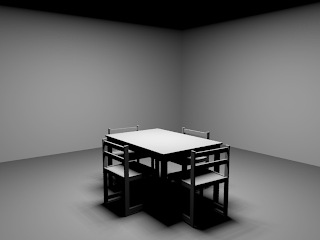
To test this implementation I used one of the scenes used by Peter Shirley for testing radiosity. The scene consists of a room with a table with chairs lit by single area light source on the ceiling. The first and second pictures show the result of rendering this scene using regular lightcuts and lightcuts extended with the implementation described above and the following settings:

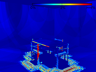
The following 2 images show the relative error (using a reference solution) for each pixel. The average relative error is 0.26% and 1.19% respectively. As expected using more tight bounds results in a relative error closer to the 2% target error.

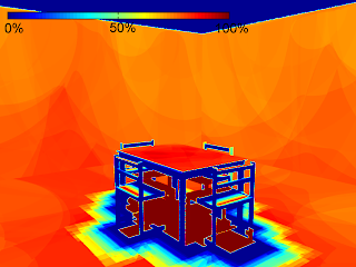
The final image shows the relative reduction in cut size for each pixel. This reduction is largest in the occluded regions where the lightcuts algorithm uses the maximum cut allowed (i.e. 1000) and the extended implementation uses a minimal cut (i.e. 1). To verify that the upper bound on its own is not the major contributor to the improvement (i.e. making the lower bound useless in this scene) I rendered this scene using only a lower and only an upper bound on the visibility. The resulting cut sizes are 82 if only a lower bound on the visibility is used and 91 if only an upper bound on the visibility is used. The upper bound is however responsible for most of the reduction in render time.
Now that is out of the way, here is what I did do:
- read some more papers on conservative visibility bounds
- implement basic visibility bounds
- Voxel Occlusion Testing: A Shadow Determination Accelerator for Ray Tracing - Woo A. & Amanatides J. (1990)
- A Survey of Visiblity for Walkthrough Applications - Cohen-Or D., Chrysanthou Y., Claudio T. S. (2000)
After reading these papers I implemented a basic lower and upper bound on the visibility. To detect clusters that are completely unoccluded (i.e. the points where a lower bound can be calculated) I used the shaft culling algorithm mention in my previous post. To verify whether a specific shaft is empty, I use a bounding volume hierarchy that is constructed during the preprocessing phase to quickly reject most primitives. The test is however conservative because it will only succeed if the entire bounding box is outside the shaft and no real primitives are tested against the shaft. Because testing a shaft is still quiet expensive, it is only used for lightcluster in the upper part of the hierarchy. In the results presented at the end of this post such test is only performed up to level 4 of the light tree which limits the number of shafts per lightcut to 31.
For detecting cluster that are completely occluded I currently use a very simple approach where one occlusion value (all lights are either occluded or not) is calculated for all cells in a regular grid. To estimate the occlusion value, a number of random rays are shot between both bounding boxes and tested for occlusion. In the results presented at the end, the scene is subdivided in 1 million cells which each use up to 1000 rays for the estimate. It is however important to notice that most cells only use a small fraction of these rays because once an unoccluded ray is found, the cell is categorized as not unoccluded. In the scene used less then 1% of maximum number of rays (1 billion) is actually tested.
To test this implementation I used one of the scenes used by Peter Shirley for testing radiosity. The scene consists of a room with a table with chairs lit by single area light source on the ceiling. The first and second pictures show the result of rendering this scene using regular lightcuts and lightcuts extended with the implementation described above and the following settings:
- resolution: 640x480
- samples/pixel: 4
- area light approx.: 1024 point lights
- render-machine: AMD X2 3800+ (single core used) with 1GB ram
- lightcuts rel. error: 2%
- max. cut size: 1000


The following 2 images show the relative error (using a reference solution) for each pixel. The average relative error is 0.26% and 1.19% respectively. As expected using more tight bounds results in a relative error closer to the 2% target error.


The final image shows the relative reduction in cut size for each pixel. This reduction is largest in the occluded regions where the lightcuts algorithm uses the maximum cut allowed (i.e. 1000) and the extended implementation uses a minimal cut (i.e. 1). To verify that the upper bound on its own is not the major contributor to the improvement (i.e. making the lower bound useless in this scene) I rendered this scene using only a lower and only an upper bound on the visibility. The resulting cut sizes are 82 if only a lower bound on the visibility is used and 91 if only an upper bound on the visibility is used. The upper bound is however responsible for most of the reduction in render time.

Wednesday, October 17, 2007
Next step?
Besides completing my Lightcuts implementation during the last week, I have searched for possible next steps in my thesis.
One possible extention to the Lighcuts algorithm, as already identified in the paper, is the addition of bounds on the visibility term. I have read a number of papers on this subject:
Further more all these techniques are quite expensive. This means they can only be used in very selective cases during lightcut calculation or only during a pre-processing phase.
The shaft-culling technique is able to efficiently detect clusters that are totally visible. This could be used to calculate lower bounds on the cluster contribution which results in better error estimates and lower cut sizes.
A totally different approach is to drop the deterministic nature of the lightcuts algorithm and use inexact estimates of the visibility. One possibility would be to first calculate a cut using the bounds and then construct a pdf over the resulting clusters using their estimated contribution. The total contribution of all lights can the be estimated by generating a number of samples from this pdf.
Ideally the user should be able to control the amount of determinism (i.e. the solution goes from the lightcuts solution to totally stochastic according to a parameter).
One possible extention to the Lighcuts algorithm, as already identified in the paper, is the addition of bounds on the visibility term. I have read a number of papers on this subject:
- Shaft Culling For Efficient Ray-Cast Radiosity - Haines E. & Wallace J. (1991)
- ShieldTester: Cell-to-Cell Visibility Test for Surface Occluders - Navazo I., Rossignac J., Jou J. & Shariff R. (2003)
- Conservative Volumetric Visibility with Occluder Fusion - Schaufler G., Julie D., Decoret X. & Sillion F. (2000)
- Ray Space Factorization for From-Region Visibility - Leyvand T., Sorkine O. & Cohen-Or D. (2003)
Further more all these techniques are quite expensive. This means they can only be used in very selective cases during lightcut calculation or only during a pre-processing phase.
The shaft-culling technique is able to efficiently detect clusters that are totally visible. This could be used to calculate lower bounds on the cluster contribution which results in better error estimates and lower cut sizes.
A totally different approach is to drop the deterministic nature of the lightcuts algorithm and use inexact estimates of the visibility. One possibility would be to first calculate a cut using the bounds and then construct a pdf over the resulting clusters using their estimated contribution. The total contribution of all lights can the be estimated by generating a number of samples from this pdf.
Ideally the user should be able to control the amount of determinism (i.e. the solution goes from the lightcuts solution to totally stochastic according to a parameter).
Saturday, October 13, 2007
Lightcuts implementation
During the past week I completed my lightcuts implementation. Concretely this means I added cosine weighted point lights and directional lights (clustering & bounds), a bound for the Blinn microfacet distribution and support for global illumination using the Instant Global Illumination algorithm as implemented in the igi plugin for pbrt.
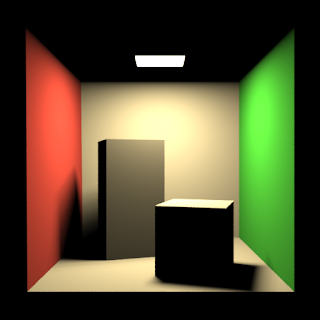
All of the following pictures where rendered using this updated implementation on my Core2 Duo T7100 system using 4 samples per pixel. The first picture is once again the cornell box but now using 1024 cosine weighted lights instead of omni directional lights with a maximum relative error of 2%. The total render time for this picture was 227s and the average cut size was 104.
The second picture shows a modified cornell box with glossy objects and global illumination. The total number of light sources used was 760000 which were mostly for the indirect light. The required time was 632s and the average cut size 206.

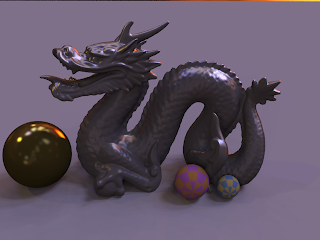
The final picture shows a glossy dragon statue lit by the grace environment map. This environment map was approximated by 256000 directional lights distributed evenly over the entire sphere of directions. The total render time was 1557s and the average cut size 218.
All of the following pictures where rendered using this updated implementation on my Core2 Duo T7100 system using 4 samples per pixel. The first picture is once again the cornell box but now using 1024 cosine weighted lights instead of omni directional lights with a maximum relative error of 2%. The total render time for this picture was 227s and the average cut size was 104.

The second picture shows a modified cornell box with glossy objects and global illumination. The total number of light sources used was 760000 which were mostly for the indirect light. The required time was 632s and the average cut size 206.

The final picture shows a glossy dragon statue lit by the grace environment map. This environment map was approximated by 256000 directional lights distributed evenly over the entire sphere of directions. The total render time was 1557s and the average cut size 218.

Subscribe to:
Posts (Atom)